Time-to-event outcome question 1: how to deal with a time-varying outcome?

Key question 1: a researcher collected data on sports injury status (in statistical terms: states) over time in a group of athletes to investigate the aetiology of Achilles tendinopathy. In weekly self-assessments, the athletes classified their injury severity into no Achilles injury, moderate Achilles tendinopathy and severe Achilles tendinopathy. The next step for the researcher is to analyse the data. Is time-to-event a suitable analytical approach to deal with a time-varying outcome?

In part 1 of the time-to-event series dealing with time-varying exposures, the idea of states, and transitions between states, was presented using Gabbett’s acute:chronic workload ratio (ACWR)15 as an example. In a similar way, sports injury (eg, Achilles tendinopathy) can be handled as a time-varying outcome. Using an example with a weekly injury classification of three states, for example, no Achilles injury (state 1), moderate Achilles tendinopathy (state 2) and severe Achilles tendinopathy (state 3) allows each athlete to be in one of these states at a specific time-point during follow-up. Then, the athlete can transit (in nine different ways) between these states during follow-up. In figure 1, the concepts of states and transitions are visualised using the three-state and nine-transition setup. Naturally, this example was made for illustrative purposes. There are other approaches to classifying injury states; however, no evidence-based guidelines support one classification model as superior over another. Therefore, the decision to use certain classification cut-offs should be based on contemporary sports theory and expert subject matter knowledge that takes into consideration the target athlete population(s). Dealing with time-varying injury-related outcomes is a highly technical and challenging task. Here, we guide the reader to further information about the specifics of multistate transitions in statistical papers.14 15

• Download figure
• Open in new tab
• Download powerpoint

Figure 1

Overview of the concepts of states, transitions and subsequent injury using an n=1 athlete example. Imagine that we register the injury status of one athlete during an 11-week follow-up. On the y-axis, the sports injury (in this case Achilles tendinopathy) can be classified into one of the three following states each week during the 11-week follow-up (marked with blue circle): state 1: no Achilles injury; state 2: moderate Achilles tendinopathy and state 3: severe Achilles tendinopathy. Then, the athlete is able to move/switch/transit between these states between each week. Consequently, the following nine multistate transitions (MST) is possible in the example: MST 1: no Achilles injury and remaining with no Achilles injury; MST 2: no Achilles injury to moderate Achilles tendinopathy; MST 3: no Achilles injury to severe Achilles tendinopathy; MST 4: moderate Achilles tendinopathy to no injury; MST 5: moderate Achilles tendinopathy and remaining with a moderate Achilles tendinopathy; MST 6: moderate Achilles tendinopathy to severe Achilles tendinopathy; MST 7: severe Achilles tendinopathy to no Achilles injury; MST 8: severe Achilles tendinopathy to moderate Achilles tendinopathy and MST 9: severe Achilles tendinopathy and remaining with a severe Achilles tendinopathy. The concept of states and transitions illustrated in the figure is directly transferable to time-varying exposures (eg, changes in training load) and time-varying effect-measure modifiers. As the athlete is classified into state 1 ‘no Achilles injury’ in week 6 and week 7, the athlete sustains two Achilles tendinopathies: the first one from week 2 to week 5 (injury 1) and the subsequent injury from week 8 to week 10 (injury 2).

If injury classification is extended beyond a dichotomised yes/no definition, standardised and/or consensus-based frameworks to systematically classify injuries into substates are needed. In a multistate framework for the analysis of subsequent injury in sport (M-FASIS), Shrier et al 10 presented a 19-state injury model classification scheme that took factors like the activity level and the treatment level into account. Although the challenges of having enough data to perform a robust statistical analysis were highlighted, the model represents an opportunity to include the concept of states (n=19) or transitions between states (n=19×19=361 transitions) using the concept of a time-varying outcome. Another example is the severity-score from the Oslo Sports Trauma Reseach Center (OSTRC) questionnaire, which is based on categorical data of 74 states between 0 and 100.11 16 Use of the OSTRC to analyse changes in injury severity implies 74 states and 5476 transitions between states. Unfortunately, an extremely large data set with many injuries would be required to analyse data in such a detailed manner. A reduction in the number of states seems necessary. To the best of our knowledge, the M-FASIS and the OSTRC are theoretical models and none has been used in a study combining time-to-event with the concept of time-varying outcomes. Still, the concepts emphasise that athletes change their injury status over time and this can be dependent on anatomical location and/or diagnoses. For these concepts, time-to-event is an appropriate analytical approach.

Importantly, the concept of multistate transition is used for the same injury type. For instance, it can be used for addressing the development of Achilles tendinopathy (eg, no Achilles tendinopathy, moderate Achilles tendinopathy, severe Achilles tendinopathy). The next step is to acknowledge that: (i) athletes can sustain the same injury multiple times during follow-up (subsequent injuries) and (ii) athletes are able to sustain other injuries than just Achilles tendinopathy (competing risk).

Key point 1: time-to-event models allow for the inclusion of time-varying outcomes using the concept of multistate transitions. To date, there is no universally accepted way to classify sports injury into different outcome states. Sports injury researchers have the opportunity to use certain injury definitions, and have a degree of flexibility to choose the cut-offs that separate each injury state.

Time-to-event outcome question 2: how to deal with subsequent injuries?

Key question 2: a researcher has collected data on subsequent injuries (eg, athletes that sustained Achilles tendinopathy three times during the follow-up). The next step for him/her is to analyse such data. Are there certain analytical approaches needed to deal with this type of data?

Finch and Cook17 developed the subsequent injury classification (SIC) model to address multiple, subsequent and exacerbation of injuries.17 During an extended follow-up period, athletes can: (i) never sustain an injury; (ii) sustain one injury or (iii) sustain more than one injury.14 In the latter case, researchers face the analytical challenge of dealing with injuries that are statistically related as they occur in the same athlete.9 12 Most likely, the risk of sustaining subsequent injuries is influenced by previous occurrences,18 hence the correlation between within-athlete subsequent injuries needs to be taken into account when analysing data.17 19 As an example, Finch et al 19 took relationships between injuries into account and found a high level of subsequent (and multiple) injuries leading to missed games in an elite athlete group.

As considerable time and resources are expended to collect these high-quality longitudinal injury data, researchers have been encouraged to make use of all of the available data.12 Unfortunately, most data analyses from these studies do not adequately address repeated injury events on the same athlete, and therefore squander its potential.12 Possibly, a reason for the limited number of analyses including multiple injuries from the same person is the complexity behind the statistical analyses. Researchers need to grasp the concept of frailty, as frailty models have been recommended for studies involving modelling of subsequent sports injury data.9 The main reason for choosing frailty models originates from their ability to correct for selection of ‘less-injury-prone’ athletes over time.20 In a 2012 paper, the frailty model was applied to rugby-related injury data to identify risk factors for contact injuries.21

Now the reader may speculate: are the concepts of multistate transitions (question 1) and subsequent injury (question 2) similar? Importantly, multistate transitions and subsequent injury should be considered two different, but nevertheless related, concepts. In figure 1, the difference between the two concepts is visualised as subsequent injury refers to injury 1 and injury 2 (marked with red), whereas each state is marked with a blue circle with arrows (representing the transitions) are connecting the states.

Key point 2: in time-to-event modelling, the researcher can consider subsequent injuries using the concept of shared frailty. This allows for correction for selection of ‘less-injury-prone’ athletes over time.

Time-to-event outcomes question 3: how to deal with competing risks?

Key question 3: in your dataset, there are data on many different injury types (eg, Achilles tendinopathy, patella-femoral pain, iliotibial band syndrome, patellar tendinopathy). However, you may only be interested in studying Achilles tendinopathy. Should you just omit all other injuries (patella-femoral pain, iliotibial band syndrome, patellar tendinopathy) when analysing the data?

In the initial presentation of the M-FASIS, OSTRC and SIC models, the possibility of dealing with multiple injuries was discussed, and the first steps were taken to promote the concept of competing risk.10 17 Standard time-to-event data include the time span from a specified time origin until the occurrence of one type of event (eg, Achilles tendinopathy).22 If there is a simultaneous risk of several types of injuries (eg, patella-femoral pain, iliotibial band syndrome, patellar tendinopathy), then these different types of injuries are considered competing, in the sense that a person can only sustain one of them at a given point in time. In the Achilles tendinopathy example, the competing risks were based on injury diagnoses. In a sports injury setting, competing risks can be assessed based on: (i) classification, for example, tendon-related injury, muscle injuries, joint-related injury and injuries unrelated to sport; (ii) anatomical location, for example, knee injury, foot injury, hip injury or (iii) diagnoses, for example, patella-femoral pain, patellar tendinopathy, Achilles tendinopathy.

To analyse competing risk data, a model describing each of these competing risks is needed. Multistate models generalise competing risk models by also describing transitions to intermediate events. Methods to analyse such models have been developed over the past three decades.23 24 Fortunately, most analyses can be performed within standard statistical software packages, but may require some extra effort with respect to data preparation and programming.22 An example from the sports injury literature that incorporates competing risks can be found elsewhere.7

The Kaplan-Meier plot, or survival curve, is recognised for its ability to visualise the probability of being injury-free (ie, surviving) or the probability of sustaining injuries (ie, not surviving) as a function of time (eg, days, weeks), training sessions or training duration.3 Importantly, Kaplan-Meier curves are no longer valid if models are extended to consider more than one type of outcome.9 23 As an example, in a competing risk setting, researchers may want to examine the probability of sustaining a tendon-related injury, with other types of injuries, such as muscle and joint-related injury and injuries occurring outside of running, being of limited interest. This presents two ways to handle data, neither of which are correct or recommended23 24:

• (i) exclude all participants who sustain non-tendon-related injury;

• (ii) include all participants who sustain non-tendon-related injury as right-censored observations at time of non-tendon-related injury (ie, ‘survived’ from a tendon injury).

In the first situation, substantial information about injury occurrences is ignored and it could appear (incorrectly) that only one type of injury, in this example, tendon injury, can occur. This is flawed since we already know that athletes are at risk of sustaining many types of injuries and that there is a statistical relationship between subsequent injuries.17–19

In the second situation, the Kaplan-Meier method computes the cumulative injury incidence proportion inclusive of the participants who are right-censored. However, this violates a principle that should be employed in time-to-event analyses: do not consider individuals as being at risk if they are injured, although a different type of injury as it can still result in them not being ‘exposed’ to risk. This will result in an overestimation of the cumulative incidence proportion as fewer athletes than appears are at risk at any one time. Consequently, statisticians have recommended researchers to include other types of injuries as competing risks and, somewhat provocatively, have also recommended researchers to ‘stick to this world’.23 In the sports science context, this essentially means that sports injury researchers who are willing to accept the assumption that injury-free athletes are only able to sustain one certain type of injury (eg, only Achilles tendinopathy) effectively ‘live in another world’.

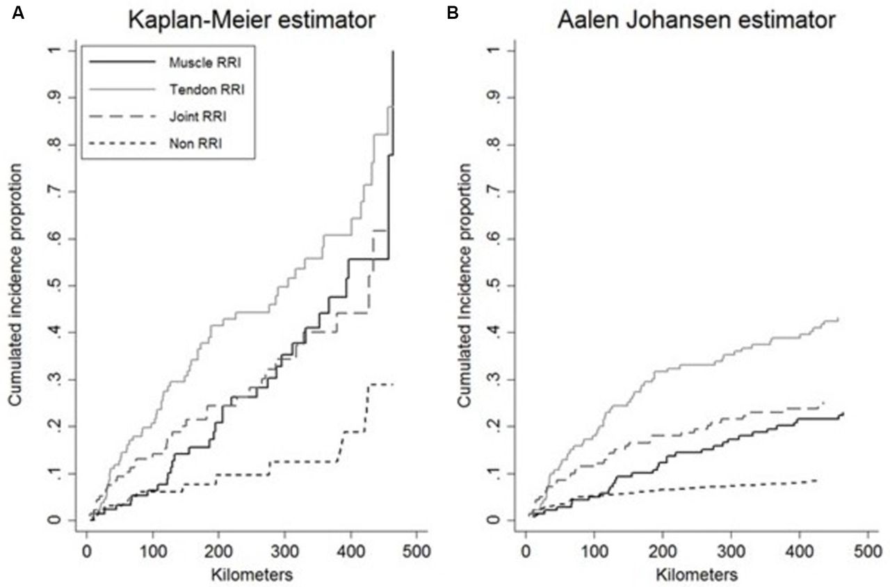
In the competing risks setting, the Kaplan-Meier method should be replaced by the Aalen-Johansen estimator to consider competing risks to avoid overestimating the cumulative incidence proportion. The difference between computing the cumulative incidence proportion using the Kaplan-Meier method (figure 2A) and the Aalen-Johansen (figure 2B) can be substantial. Using the incorrect Kaplan-Meier method in the competing risk example in figure 2A, the proportion of athletes sustaining tendon injuries is 82.1% (95% CI 65.5% to 98.8%), muscle injuries is 55.6% (95% CI 38.7% to 73.0%), joint-related injuries is 61.6% (95% CI 35.7% to 88.0%) and injuries not related to running is 29.0% (95% CI 4.2% to 53.6%). By summarising these proportions, the total proportion of athletes sustaining a first-time-injury reaches 228%. Clearly, this is impossible, since an athlete only sustains a first-time-injury once and the proportion of athletes sustaining first-time-injuries cannot possibly exceed 100%. Based on this, the proportions calculated using the Kaplan-Meier method are overestimated. Instead, the proportions reported in figure 2B, using the Aalen-Johansen estimator, are unbiased, since the total proportion of tendon injuries is 42.5% (95% CI 34.2% to 50.7%), muscle injuries is 21.6% (95% CI 14.7% to 28.4%), joint-related injuries is 25.2% (95% CI 17.9% to 32.3%) and injuries not related to running is 8.6% (95% CI 3.9% to 13.3%) does not exceed 100%. Therefore, it is strongly recommended that researchers dealing with competing risks use the Aalen-Johansen estimator as their preference.

• Download figure
• Open in new tab
• Download powerpoint

Figure 2

Kaplan-Meier vs Aalen-Johansen estimator. Comparing outputs from a flawed analysis using the Kaplan-Meier estimator (A) and a more appropriate analysis using the Aalen-Johansen estimator (B). In the former biased scenario, the proportion of athletes sustaining injury is 228%. This is impossible, since the proportion is unable to exceed 100%. In the latter scenario, the injury proportion is close to 100%. RRI, running-related injury.

Key point 3: researchers should ‘stick to this world’ by including many injury types into the analysis using a competing risk setup. Excluding injuries of less interest is strongly discouraged as it will lead to misleading results because the injury risk is overestimated.

Time-to-event outcome question 4A: how to deal with EPV

Key question 4: in the present article and in ‘Time-to-Event Analysis for Sports Injury Research Part 1: Time-Varying Exposures’, we have been enthusiastic about the potential that time-to-event modelling offers the sports injury researcher. However, in science there are always caveats and limitations. So, what are the downsides of time-to-event modelling?

One of the most important and perhaps lesser known requirements when undertaking statistical modelling of data is the EPV requirement.23 25 26 This is also known as the event/variable ratio,27 which can lead to bias if inappropriate.28 To be precise, as with any regression model, time-to-event modelling can be biased if the number of explanatory variables is large in relation to the number of injuries observed.25 28 29 In an analysis using cumulative risk difference as measure of association, the recommended number of EPVs was 10.25 A three-state version of the ACWR requires at least 20 injuries, whereas the nine transitions necessitates at least 80 injuries. Moreover, at least five injuries are required in each state/transition to avoid sparse data bias (see part B below).28 At first glance, 20–80 injuries can appear manageable for most sports injury datasets. However, for this work, we extracted the sample size from 35 studies examining training load and sports injury and identified only 11 studies with a sample size exceeding 150 participants (see table 1 in the accompanying article entitled ‘Time-to-Event Analysis for Sports Injury Research Part 1: Time-Varying Exposures’). In a 150-person study, at least half of the sample size must sustain an injury to reduce the risk of bias. Greater data collection possibilities facilitated by modern wearable technologies, such as sports watches, fitness trackers and internet-based electronic health platforms support the potential for unprecedented data collection possibilities and options for the easier recording of large data.30 When designing studies on changes in training load and injury development in the future, sports injury researchers are advised to consider EPV as a supplement to sample size or power calculations. The researcher could include more athletes into the study. Another (or supplementary) approach would be to extend the follow-up period to capture a greater number of injuries.

We note that EPV considerations do not account for other contributing factors to sparse data bias such as explanatory variables with narrow distributions or with categories that are very uncommon,28 31 nor do they consider the impact of the commonly used stepwise variable selection approach which requires even more EPV than do models with prespecified variables. A better diagnostic for sparse data bias is to repeat the analysis using mild shrinkage or penalisation methods: substantial changes warn of serious bias in the original estimates.28 31 32

Key point 4A: sports injury researchers need to calculate the event/variable ratio to avoid biased results.

Time-to-event outcome question 4B: how to deal with number of injuries in each exposure state?

In addition to the EPV requirements, all exposure states and/or transitions in the analysis must include at least five events to conduct a robust statistical analysis. In table 2, the cumulative incidence proportion for different states of two exposure variables (changes in running distance and change in running intensity) are presented as an example of a result based on a flawed time-to-event. Clearly, the cumulative injury incidence proportions of −7.6% and −18.9% are flawed as an injury incidence proportion can never reach a value below 0%. Consequently, sports injury researchers working with time-to-event analyses are encouraged to show the number of injuries in each exposure state to enable readers to assess the robustness of the models presented. If the number of injuries in a certain state is below five, analysts should carefully consider reclassifying their data based on other cut-offs or reducing the number of states used in the analysis.

With these considerations in mind, time-to-event statistical modelling can offer a range of opportunities for researchers to include exposure variables, such as changes in training load (either as states or transitions), across the course of a study.

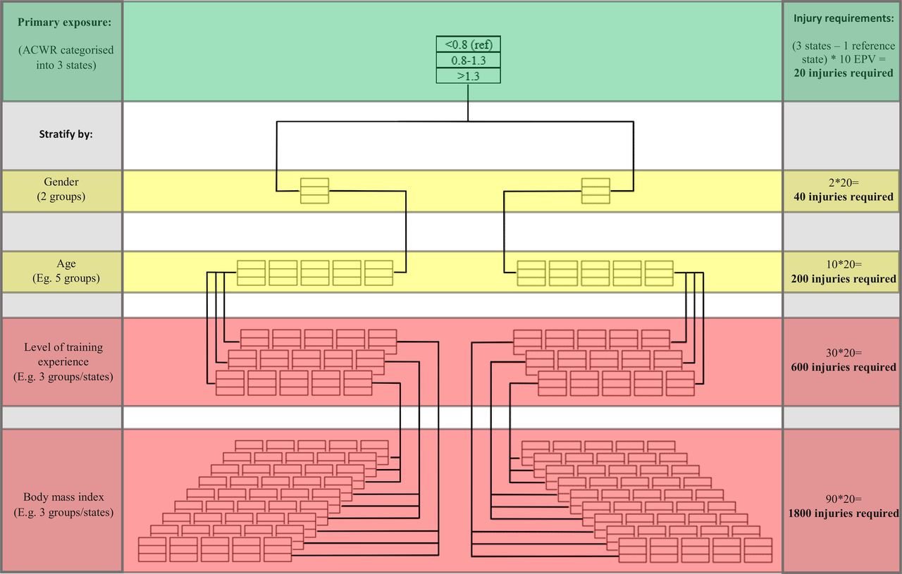
The concept of sparse data bias has implications for future research in sports injury aetiology. The requirement forces sports injuries to be evenly distributed across the states or transitions if the requirements behind the analysis are to be fulfilled. As visualised in figure 3, this requirement becomes particularly difficult to accommodate when a stratified analysis is required as the number of variables increases exponentially for each additional strata included. Do we consider stratified analysis in a sport injury setting, you may ask? Certainly, stratified analyses are needed if the aim is to answer the question: ‘how much change in training load is too much before injury is sustained, among athletes with different characteristics?' Responding to this question using multiple time-varying exposures (and outcomes) requires many injuries. In figure 3, an example is provided that visualises why many injuries are needed. This should not be a barrier for future research, but collaborations across borders to collect the amount of data needed seem to be an important step forward.33

• Download figure
• Open in new tab
• Download powerpoint

Figure 3

Stratification requires many injuries. Injury (event) requirements according to (i) a crude analysis (top green) and (ii) when including one (top yellow), two (bottom yellow), three (top red) or four (bottom red) effect-measure modifiers. In the examples, the number of injuries (events) required in a time-to-event analysis is calculated based on a cumulative risk difference (CRD) as measure of association. If other measures of association are used, the numbers could differ. In the crude analysis using acute:chronic workload ratio (ACWR) categorised into 3 states (<0.8, 0.8–1.3 and >1.3) as primary exposure (top, green), a total of 20 injuries are needed since (3 states–1 reference state)×10 injuries (events) per variable (EPV)=20. If the analysis is extended to include one effect-measure modifier (top yellow), 40 injuries are required (20 injuries in each gender-strata). If four effect-measure modifiers are included (bottom red), eg, gender (2 time-fixed groups), age (eg, 5 time-fixed groups), level of training experience (eg, 3 time-fixed groups or time-varying states) and body mass index (eg, 3 time-fixed groups or time-varying states), the total number of injuries required reach 1800 injuries (20 injuries in each of the 90 substrata).

Key point 4B: sports injury researchers should ensure there are at least five injuries in each exposure state to be analysed. Dealing with (multiple) time-varying exposures requires a considerable number of injuries to avoid violating the requirements underpinning the time-to-event analysis. Analysing data without consideration to number of injuries in each exposure state will easily lead to sparse data bias.

Time-to-event outcomes question 5: are there considerations when designing my study?

Key question 5: I want to design a new study looking into the association between changes in training load and sports injury. What should I consider when I am designing my data collection?

In the previous section, we presented important assumptions and requirements underpinning the analysis when dealing with the research question 'how much change in training load is too much before sports injury is sustained, among athletes with different characteristics?' We argued that careful attention to the EPV requirement and having at least five injuries in each exposure state is needed to avoid biased results. From experience, we have learnt that many researchers do not consider these requirements.

In most prospective sport injury studies, fewer than 1000 athletes or participants have been included (see table 1 in the accompanying article entitled ‘Time-to-Event Analysis for Sports Injury Research Part 1: Time-Varying Exposures’). Although the workload needed to logistically handle this number of participants is considerable and time-consuming, advanced data analyses involving multiple time-varying exposures and a time-varying injury outcome can literally necessitate tens of thousands (or possibly millions) of athletes to experience a sufficient number of injuries to avoid sparse data bias.28 This issue has been noted in the wider epidemiological literature.34 35 Sports injury researchers cannot always conduct the most rigorous study and/or satisfy the theoretic and practical requirements that are necessary to undertake a robust statistical analysis. However, in situations when it is financially and logistically possible to design and conduct a high-quality, large-scale epidemiological cohort study, researchers should make a concerted effort to consider and implement the necessary principles and directives discussed in this article. Moreover, to appropriately advance the science of sports injury control and prevention, sports injury researchers are expected to question assumptions underpinning statistical analyses and ask whether there are better ways of analysing data, and asking ‘the right’ questions while equally challenging contemporary aetiological theories. In doing so, advanced statistical approaches such as time-to-event analyses that are widely used in other disciplines and health science contexts can be raised to the same level of application and scrutiny for sports injury research. Time-to-events analyses offer a range of opportunities regarding modelling approaches (Cox regression vs pseudo-observation method), measure of association and graphical presentations. As these concepts have been presented elsewhere,3 an extensive description is not provided. However, the informed reader is provided with an overview of the opportunities in table 3.

Key point 5: researcher must consider: am I able to get the number of injuries needed in order to analyse changes in training load as a time-varying exposure to sports injury? How many injuries are likely to occur in each exposure state (or transition)? How many cut-offs to separate the exposure groups are suitable?

Time-to-event outcomes question 6: are there alternative methods?

Key question 6: it is difficult to collect the amount of data needed to avoid violating the assumptions and requirements needed to perform a robust time-to-event analyses on a change in training load-related question. Accordingly, are there any alternative methods that could be considered?

Complex systems and computational modelling have received more attention in the sports injury science literature recently.36 These methods are complementary to traditional statistical modelling and time-to-event analyses. In a small sample setting or in the absence of large-scale data, alternative computational systems science methods, including simulation-based techniques, could be considered alongside, or integrated with, traditional statistical approaches.36 For example, the use of agent-based modelling (ABM) has been recently promoted and discussed as a complementary method for sports injury research.37 Specifically, ABM is a form of computational science that involves modelling the behavioural dynamics of individual micro-entities known as ‘agents’. These agents can interact with one another and learn over time based on past experiences; update their internal ’states' autonomously and/or create global patterns of behaviour. In relation to both time-to-event modelling and sports injury aetiology, the clear advantage of ABM lies in its capability to model hundreds or thousands of athletes, of whom can be assigned real-world demographics (eg, age), biologic (eg, sex), lifestyle (eg, diet) and/or training-related (eg, primary workload exposure) characteristics.37

We have demonstrated in this paper that in order to conduct a robust statistical sports injury analysis and avoid sparse data bias, the number of injuries observed in each exposure state (or transition) should exceed 5. Accordingly, the flexibility of ABM and other simulation-based techniques could offer a potential workaround to the requirements in traditional statistical analyses, especially when sports injury researchers aim to further stratify samples to prioritise and understand how workloads and other time-varying exposures change status during follow-up.30 38 39 With continued application and ingenuity, computational simulations might be able to capture a sufficient number of sports injuries per explanatory variable modelled, affording theoretical insight into the supposed aetiologic mechanism(s). Despite the versatility of computational methods, a word of caution is advised. Unlike traditional statistical modelling, the assumptions underpinning computational models are often based on subject matter knowledge and other various forms of empirical evidence. Thus, the underlying data-driven assumptions and theoretical causal mechanisms encoded into simulations should be explicitly described as a basis for evaluating model predictions.34 35

Key point 6: the use of computational modelling could be considered as a complementary and alternative approach to time-to-event modelling in future sports injury research applications because no considerations to number of injuries is needed. However, unlike traditional statistical modelling, the assumptions underpinning computational models are often based on subject matter knowledge and other various forms of empirical evidence. If these are wrong, the results from the analyses will be questionable.