In many epidemiological and medical studies, the outcome variable of interest is a recurrent event. Among others, low back pain, sickness leave from work, sporting injuries, and hospitalisation are examples of recurrent events that are often reported.^1,2 Basically, the different statistical techniques to analyse recurrent event data can be divided into naive techniques and longitudinal techniques. Naive techniques are characterised by either ignoring the existence of recurrent events or ignoring the fact that the recurrent events within subjects or patients are correlated. Longitudinal techniques on the other hand are characterised by the fact that the whole pattern of recurrent events over time is analysed, taking into account that the recurrent events are correlated within subjects or patients. Despite the fact that there are many statistical techniques available to analyse recurrent event data,³ for most researchers it is rather difficult to choose the proper technique to answer the research question they are interested in. Reviewing the literature, it is rather surprising that most authors use naive statistical techniques to analyse their study outcomes.⁴ A possible explanation for this is that most longitudinal techniques are only described in specific statistical literature, which is difficult to understand for most (non-mathematical) researchers.^5,6 However, the general ideas behind these techniques are not as difficult as often suggested.

Therefore, the purpose of this paper is threefold: (1) to give an overview of easily applicable statistical techniques that are available to analyse recurrent event data, (2) to compare the results of naive and longitudinal techniques with each other, and (3) to give some recommendations on how to analyse recurrent event data, given a certain research question.

METHODS

Study design

The data used in the example are from a study of Smidt et al.⁷ They investigated the effectiveness of corticosteroid injections, physiotherapy, and wait and see policy for lateral epicondylitis in a randomised controlled trial in primary care. In this study patients who consulted one of 85 participating general practitioners for elbow complaints were considered for participation in the study. The eligible patients were allocated at random either to a wait and see policy (n = 59) to corticosteroid injections, (n = 62) or to physiotherapy (n = 64). The outcome variable used in this example was treatment success. Treatment success was based on general improvement, which was scored on a six point Likert scale (completely recovered to much worse). Patients who rated themselves as completely recovered or much improved were considered as a treatment success. The outcome variable was assessed once during the intervention period (after three weeks), just after the intervention period (after six weeks), and 12, 26, and 52 weeks after randomisation. For detailed information regarding the intervention the reader is referred to Smidt et al.⁷

Statistical analysis

Descriptives

First of all, an overview is given of the different response patterns regarding the outcome variable treatment success observed in the example study. Secondly, the proportion of subjects with treatment success at each time point is graphically presented.

Naive techniques

In this paper, two frequently used naive statistical techniques to analyse recurrent event data are presented. The techniques are naive in such a way that they do not use all available data, but only one observation for each patient. Firstly, a logistic regression analysis is performed to analyse the difference in the proportion of patients with treatment success at the end of the study—that is, at 52 weeks. Secondly, a survival analysis (that is, Cox proportional hazards regression) is performed with the first experienced event (treatment success) and the time to that event as outcome variable.

Longitudinal techniques

The difference between the naive techniques, and the longitudinal techniques is that with the longitudinal techniques not one observation for each patient is used, but that all observations for each patient are used in the analysis. This implicates directly that a so called long data structure is needed to perform these kind of analyses (see table 1).

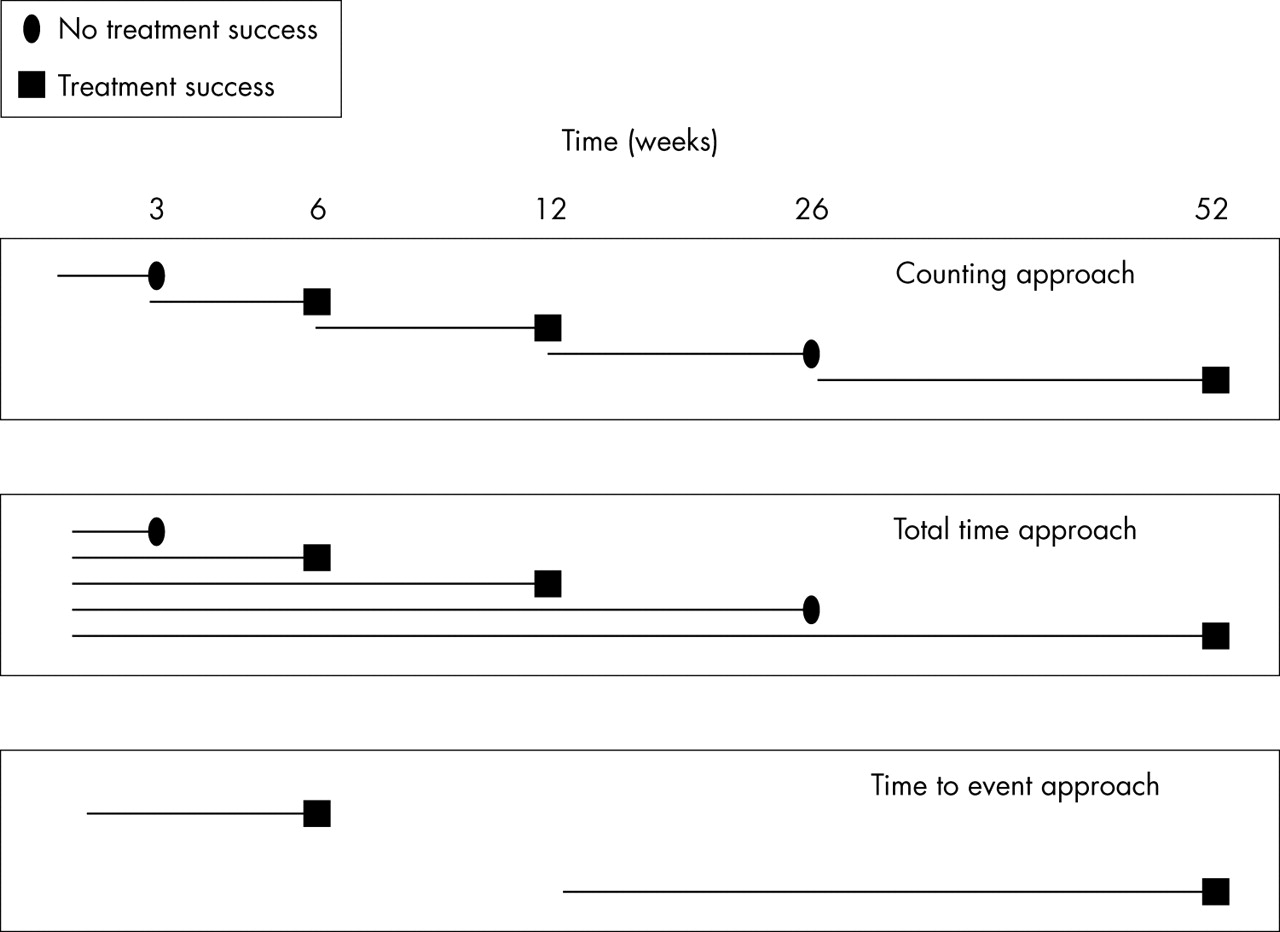
In such a long data structure there is more than one record present for each patient. The general idea behind all longitudinal techniques is that because of the dependency of observations within a patient a correction must be made for patient. The problem, however, is that patient is a categorical variable that must be represented by dummy variables. In the example dataset there are 185 patients, so 184 dummy variables are needed to correct for patient. Because this is practically impossible, the correction for patient has to be done in a different way and the different longitudinal techniques differ from each other in the way they perform that correction. The longitudinal techniques can be further divided into survival approaches and (longitudinal) logistic regression approaches. Regarding survival approaches, Cox proportional hazards regression for recurrent events was performed. Although there are different estimation procedures available,⁸ the general idea behind Cox proportional hazards regression for recurrent events is that the different time periods are analysed separately adjusted for the fact that the time periods within one patient are dependent.⁹ The idea of this adjustment is that the standard error of the regression coefficient of interest is increased proportional to the correlation of the observations within one patient. One of the problems using Cox proportional hazards regression for recurrent events is the question how to define the time at risk. Especially in this example, because the events under study are not short lasting events, but can be long lasting—that is, continuing over more than one time point (that is, they can be considered as states). For illustrative purposes, in this example the time at risk is defined in three different ways (see fig 1): (1) the counting approach. Each time period is analysed separately assuming that all patients are at risk at the beginning of each period, irrespective of the situation at the end of the foregoing period, (2) the total time approach. Comparable to the counting approach. However, in the total time approach, the starting point for each period is the beginning of the study, (3) the time to event approach. In this approach only the transitions from no treatment success to treatment success are taken into account. So, if for a patient the treatment was successful after three months and stays successful at all repeated measurements, only the first time is taken into account in the analysis. When for another patient the treatment was successful after three months, and reports not successful at six months, that particular patient is again at risk from three months onwards until the treatment for that patient is successful for the second time, or until the follow up period ended.

Regarding the logistic regression approaches two techniques are used to analyse the recurrent event data: generalised estimating equations (GEE analysis),^10,11 and random coefficient analysis, which is also known as multilevel analysis.^12,13 Again, both methods are regression methods taking into account the fact that the observations within one person are dependent. The difference between the methods is that they make this correction in a different way. Within GEE, this correction is performed by adding a correlation matrix to the regression model, which exists of an estimation of the correlations between the different time points within one patient. Depending on the software package used to estimate the regression coefficients, different correlation structures are available. They basically vary from an exchangeable (or compound symmetry) correlation structure (that is, the correlations between subsequent measurements are assumed to be the same, irrespective of the length of the interperiod) to an unstructured correlation structure. In this structure no particular structure is assumed, which means that all possible correlations between repeated measurements have to be estimated.¹⁰

It has been mentioned before that it is impossible to correct for patient by adding dummy variables to the regression model. Adding a dummy variable for each patient to a regression model, actually means that for each patient a different intercept is estimated. The basic idea behind the use of random coefficient analysis in longitudinal studies is that not all separate intercepts are estimated, but that (only one) variance of those intercepts is estimated—that is, a random intercept. It is also possible that not only the intercept is different for each patient, but that also the development over time is different for each patient, in other words, there is an interaction between patient and time. In this situation the variance of the regression coefficients for time can be estimated—that is, a random slope for time.¹²

The naive statistical analyses, Cox regression analyses for recurrent events and GEE analyses were performed with Stata,¹⁵ and random coefficient analyses were performed with MLwiN¹⁶ (see appendix available on line http://www.jech.com/supplemental).

RESULTS

Table 2 gives an overview of the different response patterns observed in the patients with lateral epicondylitis. This table shows for instance that in the wait and see group, seven patients did not report any treatment success along the whole follow up period, while for the injection group and the physiotherapy group these numbers were respectively none and one. This table also shows that in the wait and see group, three patients report a treatment success after three weeks, which continues over the whole follow up period of 52 weeks. For the injection and physiotherapy group these numbers were higher (11 and 8 respectively). Finally, the table shows that especially in the injection group the observed response patterns are very unstable.

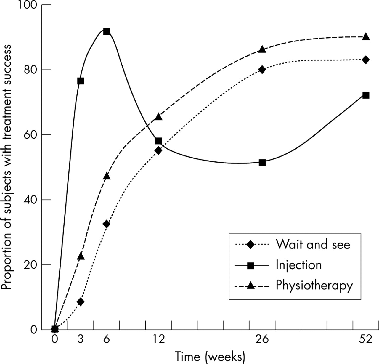
Figure 2 shows the development over time regarding the proportion of patients with treatment success. A sharp increase for the injection group in the first six weeks is followed by a sharp decrease to 12 and 26 weeks, whereafter the development is more or less equal to the development of the two other groups. The other two groups increase gradually over the whole follow up period, although the physiotherapy group is slightly better than the wait and see group.

Table 3 shows the results of the different analyses performed. In all analyses the injection group showed the highest odds ratio or hazard ratio, except for the logistic regression analysis performed on the data at 52 weeks. In the latter, the odds for treatment success for the physiotherapy group was higher than the one for the wait and see group, but this difference was not statistically significant. Regarding the hazard ratios for the different Cox regression for recurrent events, the results were comparable, although the time to event approach showed a somewhat higher hazard ratio for the injection group compared with the other two approaches. Regarding the two longitudinal logistic regression techniques (GEE analysis and random coefficient analysis), the odds ratios estimated with random coefficient analysis were much higher than the ones estimated with GEE analysis, although with both techniques the injection group performed better than the physiotherapy group and both were significantly better than the wait and see group.

DISCUSSION

One of the purposes of this paper was to provide an overview of different techniques that can be used for the analysis of recurrent event data. The simplest and probably most illustrative way of describing recurrent event data is plotting the proportion of subjects recovered at each time point (see fig 2) or showing the different response patterns observed (see table 2). Although both can give a nice overview, it is difficult to analyse the patterns of this figure statistically. So, therefore, several statistical analyses were performed on the recurrent event data. Most striking is that the techniques that use all available data show totally different results than the techniques that use only part of the data. In fact, although all three Cox regression approaches as well as the GEE analysis and the random coefficient analysis are strongly in favour of the corticosteroid injection group, the authors of the original paper recommend either a wait and see policy or physiotherapy treatment. This recommendation was highly based on their interest in the long term effect of the interventions—that is, using the results of the logistic regression analysis at week 52. This directly emphasises the importance of the research question. With the logistic regression analysis using the data assessed at 52 weeks, the long term effect of the intervention is analysed, while with the naive Cox regression analysis the short term effect of the intervention is analysed. With the longitudinal techniques that use all available data, the overall intervention effect—that is, the whole development over time is analysed. A different research question leading to totally different results.

Looking at the three Cox regression analyses for recurrent events, the hazard ratio for the injection group was somewhat higher for the time to event approach then for the other two approaches. This has everything to do with the number of transitions in the injection group. Suppose that the treatment for a patient was successful after three weeks and stays successful for the rest of the follow up period, only one event is considered with a time at risk of three weeks. Suppose that for another patient the treatment was also not successful after three weeks, but was successful at six weeks and 12 weeks, not successful at 26 weeks and successful again at 52 weeks, for that patient two events are considered with respectively six and 40 weeks of time at risk (see fig 1). When analysing these two subjects with a time to event approach, the second patient will do better than the first, which is rather strange and in fact not true. So, in a situation with a lot of transitions the time to event approach must be interpreted cautiously.

The two longitudinal techniques, GEE analysis and random coefficient analysis, lead to different results. Basically, both longitudinal techniques take all measurements of successful treatment and not successful treatment into account, and use a logistic regression approach with a correction for the dependency of the observations. The difference between the two techniques is that GEE analysis is a so called population average approach, while random coefficient analysis is a so called subject specific approach.^17,18 The different estimation procedures cause the difference in the magnitude of the odds ratios, which is always in favour of the random coefficient analysis—that is, the effects estimated with random coefficient analysis are always bigger than the effects estimated with GEE analysis.^17,18 It should also be noted that the estimations of the regression coefficients (that is, odds ratios) with random coefficient analyses of recurrent events can be very complicated and often lead to instable results. Furthermore, the results of these analyses can differ between software packages.^18–20

An advantage of using a Cox regression approach is that hazards ratios (interpretable as relative risks) are estimated, while with logistic regression approaches, odds ratios are estimated. Especially in experimental research where the proportion of subjects experiencing an event is comparatively high (as in the present example), the odds ratio is an overestimation of the real relative risk. This also explains the fact that the magnitude of the odds ratios estimated with GEE and random coefficient analysis are higher than the hazards ratios estimated with Cox regression for recurrent events.

An important problem of using Cox regression for recurrent events on the other hand is the assumption of proportional hazards over time. An assumption that does not hold in many situations. When the proportional hazards assumption does not hold, it is possible to divide the follow up period into several sub-periods and calculate different hazard ratios for each sub-period. Furthermore, compared with the longitudinal logistic regression approaches (that is, GEE analysis and random coefficient analysis) the possibilities to correct for the dependency of observations in using Cox regression are rather limited. In fact the correction only influences the standard error of the regression coefficient—that is, the width of the 95% confidence interval around the hazard ratio. The point estimate is equal to the point estimate derived from an analysis when the observations are considered to be independent.

Although the example is a quite common situation, it should be taken into account that it is different from a recurrent event situation, in which the events are short lasting.⁸ In the study presented in this paper, the events are not short lasting, but they can be more or less considered as states (they are long lasting relative to the total follow up time). Some of the patients’ treatments are successful at a certain time point and stay successful until the end of the study. When the duration of the events under consideration is short relative to the total follow up time, the definition of the time at risk for a Cox regression for recurrent events is somewhat easier than in this example.

Another issue that should be taken into account is that the measurements in this example are performed on predefined time points. Although this is the situation in most experimental studies, it is also possible to measure on a continuous time scale (for example, when outcomes such as sick leave from work or hospitalisation are considered). This basically means that measurements are taken exactly at the moment the event of interest occurs. Therefore, the number of measurements per subject or patient and the spacing of these measurements are highly dependent on the number and spacing of the recurrent events. In these situations the definition of the time at risk can be slightly different from the ones described in this example.⁴ It should further be noted that in a situation when time is measured on a continuous scale, longitudinal techniques such as GEE and random coefficient analysis are not suitable, unless all time points and events that occur are considered as measurement points.

General comments

One of the purposes of this paper was to give an overview of (comparatively simple) easily applicable statistical techniques to analyse recurrent event data. Therefore, in these examples, the models are as simple as possible. However, all analyses presented can be easily extended with both time independent and time dependent covariates. The latter, of course, only in the situations where the development over time is analysed.

The example used in this paper is from a randomised controlled trial. However, the longitudinal techniques to analyse recurrent event data can also be applied to observational cohort studies. Because the techniques are either an extension of Cox proportional hazards regression or logistic regression, issues as effect modification and confounding can be handled in exactly the same way as in the classic application of these techniques. Of course, because of the longitudinal nature of the data, possible effect modifiers or confounders can be time independent as well as time dependent. The biggest difference between a randomised controlled trial and an observational cohort study is probably the fact that within an observation cohort study, patients can have a certain event already at baseline. This implicates that Cox regression for recurrent events is not really suitable in observational studies where this occurs.

The study used as an example is a study with single type event data. Only one kind of event (treatment success) is used as outcome. Although the interpretation of the results is slightly different, it is obvious that the same kind of approaches as described in this paper can be used for analysis of multi-type event data such as tumours at different sites, different kinds of infection, etc.²¹

Recommendation

The way recurrent event data is analysed highly depends on the research question of interest. If you are only interested in a particular short term or long term result, simple techniques are highly appropriate. However, if the development of a particular outcome is of interest, statistical techniques that consider the recurrent events and additionally correct for the dependency of the observations are necessary to answer the accompanying research question. When discrete time points are analysed, GEE analysis or random coefficient analysis can be used, but GEE is recommended because of the population average approach and the comparatively simple estimation procedures compared with random coefficient analysis. When the events can occur continuously, Cox proportional hazards regression for recurrent events must be used, but special attention has to be given to the definition of the time at risk and to the assumption of proportional hazards.