Article Text

Abstract
Objective To characterise the time course of changes in haemoglobin mass (Hbmass) in response to altitude exposure.
Methods This meta-analysis uses raw data from 17 studies that used carbon monoxide rebreathing to determine Hbmass prealtitude, during altitude and postaltitude. Seven studies were classic altitude training, eight were live high train low (LHTL) and two mixed classic and LHTL. Separate linear-mixed models were fitted to the data from the 17 studies and the resultant estimates of the effects of altitude used in a random effects meta-analysis to obtain an overall estimate of the effect of altitude, with separate analyses during altitude and postaltitude. In addition, within-subject differences from the prealtitude phase for altitude participant and all the data on control participants were used to estimate the analytical SD. The ‘true’ between-subject response to altitude was estimated from the within-subject differences on altitude participants, between the prealtitude and during-altitude phases, together with the estimated analytical SD.
Results During-altitude Hbmass was estimated to increase by ∼1.1%/100 h for LHTL and classic altitude. Postaltitude Hbmass was estimated to be 3.3% higher than prealtitude values for up to 20 days. The within-subject SD was constant at ∼2% for up to 7 days between observations, indicative of analytical error. A 95% prediction interval for the ‘true’ response of an athlete exposed to 300 h of altitude was estimated to be 1.1–6%.
Conclusions Camps as short as 2 weeks of classic and LHTL altitude will quite likely increase Hbmass and most athletes can expect benefit.
- Altitude
- Statistical review
This is an Open Access article distributed in accordance with the Creative Commons Attribution Non Commercial (CC BY-NC 3.0) license, which permits others to distribute, remix, adapt, build upon this work non-commercially, and license their derivative works on different terms, provided the original work is properly cited and the use is non-commercial. See: http://creativecommons.org/licenses/by-nc/3.0/
Statistics from Altmetric.com
Introduction
An increase in erythropoiesis resulting from altitude exposure has been described for over 100 years,1 and is quite apparent among lifelong residents of high altitude (>3000 m).2–4 However, for short-term sojourns, a comprehensive new meta-analysis and Monte Carlo simulation of data spanning the last 100 years concluded that there was no statistically significant increase in red cell volume (RCV) unless the exposure exceeded 4 weeks at an altitude of at least 3000 m.5 This altitude is substantially higher than that recommended for athletes,6 where a lower altitude (2000–2500 m) is advised to minimise the loss of training intensity evident at higher elevations. Rusko et al7 have suggested that an exposure of 3 weeks is sufficient at altitudes >∼2000 m, provided the exposure exceeds 12 h/day. Furthermore, Clark et al8 have concluded, based on the serial measurements of haemoglobin mass (Hbmass) and on other recent altitude studies, that Hbmass increases at a mean rate of 1%/100 h of exposure to adequate altitude.
Rasmussen et al,5 who were careful in the selection criteria for studies to include in their meta-analysis, noted that a variety of methodologies to measure RCV were adopted in the different studies, ranging from carbon monoxide (CO) rebreathing to radioactive labelling of albumin to various plasma dye-dilution tracer methods. As with any meta-analysis, the veracity of the conclusions is only as good as the quality of the data included, and Rasmussen et al formally tested that there was no significant effect of the method of measurement on their conclusions. However, all methods of estimating RCV or Hbmass are subject to error, and a meta-analysis of raw data demonstrated that the measurement error of CO rebreathing (2.2%) was, if anything, slightly less than that (2.8%) for the gold standard method of 51chromium-labelled red blood cells.9 In contrast, the measurement error for the common plasma dilution method of Evans Blue dye was estimated to be 6.7%. If the effects of moderate altitude (2000–3000 m)10 are relatively small, then it is quite likely that inclusion of studies with greater error (eg, refs. 11 and 12) may obfuscate the effects of studies using more reliable methods (eg, refs. 13 and 14).
In 2005, Schmidt and Prommer15 validated a variation on the CO rebreathing method with a low error of measurement of ∼1.7%, which has been successively refined.16–18 Thus, rather than using many data sources, some of which include relatively noisy data, the aim of this meta-analysis was to use the raw data of only those studies that used the optimised CO rebreathing method to determine Hbmass, and that were conducted since 2008. This approach should offer a more precise estimate of the effect of altitude on Hbmass.
Methods
Data sources
The data used in the meta-analysis were obtained from authors who had, since 2008, published the results of studies that used the ‘optimised CO rebreathing’ method to evaluate the effects of altitude training on Hbmass. Briefly, this rebreathing method involves a known CO dose of ∼1.2 ml/kg body mass being administered and rebreathed for 2 min. Capillary fingertip blood samples are taken before the start of the test and 7 min after administration of the CO dose. Both blood samples are measured a minimum of five times for determination of percentage of carboxyhaemoglobin (%HbCO) using an OSM3 Hemoximeter (Radiometer, Copenhagen). Hbmass is calculated from the mean change in %HbCO before and after rebreathing CO.
Individual, deidentified raw data were provided from 17 studies8 ,13 ,14 ,19–31; seven were classic altitude training (ie, living and training on a mountain) studies,13 ,22 ,23 ,28 ,29 ,31 ,32 eight were live high train low (LHTL) studies8 ,14 ,19–21 ,25 ,27 ,30 and two included a mixture of classic and LHTL modalities.24 ,26 Regardless of the form of altitude or simulated altitude, hereafter, all such studies will be referred to as ‘altitude’ studies for simplicity.
Coding of predictor variables
Altitude treatments
In addition to the recorded altitude of each study, the total hours spent in hypoxia was calculated from the hours per day and numbers of days of exposure. This approach allowed for comparison of classic and LHTL modes, since the former affords continuous altitude exposure, while the latter is intermittent. All but one of the LHTL studies used ≥14 h/day in hypoxia, while the other used 10 h/day.24 Several of the classic and LHTL studies made serial measurements of Hbmass during altitude exposure (table 1), which enabled multiple estimates of the change in Hbmass over time. All studies included prealtitude and postaltitude measurements of Hbmass.
Data sources
Where included in the study design, control participants were coded as controls and those exposed to altitude were coded as altitude participants. The one exception was the LHTL study of Neya et al24 where the control group resided at 1300 m 24 h/day; these participants were coded as classic altitude, albeit at the lowest altitude of any group and very much lower than that conventionally associated with an increase in RCV.33
Statistical analysis
The approach taken was first to fit linear mixed models separately to the data from each of the 17 studies to estimate the effects of altitude. The resultant estimates were then used in a random effects meta-analysis to obtain an overall estimate of the effect of altitude, with separate analyses for the during-altitude and postaltitude phases. In addition, all possible within-subject differences for control participants and those during the prealtitude and during-altitude phases for altitude participants were used to evaluate within-subject variation. All analyses were conducted using the statistical package R,34 with the mixed model analyses conducted using the mle procedure available in R's nlme library.35
In the initial analyses of the 17 studies, Hbmass values were log transformed (natural logarithms (ln)) and linear mixed models fitted with treatment (control or altitude), days during altitude, days postaltitude and sex as fixed effects and participant as a random effect. In addition, where appropriate, the models allowed for different within-subject SDs for men and women (some of the studies used all male or all female participants) and within-subject autocorrelation. Some of the studies had too few observations on each participant to warrant inclusion of the assumed autocorrelation structure but, for consistency, the same form of model was fitted to all 17 data sets.
The next stage fitted linear mixed models with response variable estimates of the mean (over participants within each study) differences between baseline and subsequent values of ln(Hbmass) on altitude participants, with separate analyses for the during-altitude and postaltitude phases.
For the during-altitude phase, the time at altitude, both in terms of the number of days and the number of hours, the altitude and the type of altitude (classic or LHTL) were treated as fixed effects; whereas for the postaltitude phase, altitude, the number of days and hours at altitude, the type of altitude and number of days postaltitude were treated as fixed effects. For both analyses, the study was treated as a random effect and the SEs associated with the estimates of mean differences, as provided by the initial analyses, were used to determine suitable weightings.
Estimates obtained from these analyses were back transformed (via the exponential function) to express results as percentage changes on the Hbmass scale.
Variability of measurements
Without some form of intervention, Hbmass is considered to be constant, especially over a period of a few days, so that differences in measurements taken under stable conditions can be attributed almost exclusively to measurement, or analytical, error.36 Using the within-subject variability of the recorded Hbmass values among the control participants and the within-subject variability during (just) the prealtitude phase among the altitude participant, it is possible to estimate the magnitude of the analytical error. In addition, following Hopkins,37 it is also possible to estimate the overall magnitude of between-subject differences in response to altitude training using the within-subject differences in Hbmass measurements between the prealtitude and during-altitude phases, and between pairs of during-altitude measurements, made on the altitude participants.
Within-subject measurements
Using the control participant data and just the prealtitude values from altitude participants, an estimate of the analytical SD was obtained as follows. Separately for each study, estimates of within-subject SDs associated with each difference in days were obtained as the square root of half the average of the squared differences in ln(Hbmass). A linear mixed model was then fitted to the ln-transformed (estimated) SDs with the number of days between estimates as a fixed effect, study as a random effect and weights determined by the numbers of differences used to estimate the SDs. The results of this analysis were back transformed (twice, using exponentials) to obtain coefficients of variation (CVs) on the Hbmass scale, with the analytical CV estimated as the value associated with readings zero days apart.
Between-subject ‘true’ responses
Using data from (just) the altitude participants, estimates of the between-subject variation in the ‘true’ response to altitude were obtained as follows. First, estimates of the within-subject SDs of ln(Hbmass) associated with differences between prealtitude and altitude values, and between values obtained while at altitude, for different values of the difference in the number of hours at altitude, were obtained as the SD of the relevant differences divided by √2. Linear mixed models were then fitted to the ln-transformed SDs with the difference in the number of hours at altitude as a fixed effect, study as a random effect and weights determined by the degrees of freedom of the estimated SDs. The models considered were constrained so that the estimated within-subject SD after zero (additional) hours at altitude agreed with the estimate of the analytical SD. This was achieved by subtracting the natural log of the estimated analytical SD from each of the ln-transformed SDs and then fitting models without an intercept term. Estimates of the SDs of the between-subject ‘true’ responses were then obtained as
for a range of values of (differences in) the hours at altitude; these SDs were then used to estimate the likely range of ‘true’ responses to different exposures to altitude.
Results
Raw data
A total of 1624 measures of Hbmass were made on 328 participants, 18 of whom participated in more than one study (14 in 2 studies, 3 in 3 studies and 1 in 4 studies); 225 participants participated as altitude-only participants, 96 as control-only participants and 7 as altitude and control participants, but in different studies (table 1). The mean (±SD) number of measures per participant was 4.8 (±2.7). As the serial measures were made virtually during all studies, there were 76 estimates of the change in ln(Hbmass) from the prealtitude values, 40 estimates during altitude and 36 estimates after altitude exposure.
The median classic altitude was 2320 m (range 1360–3600 m); while all but one LHTL study used 3000 m, the other used 2500 m.
During altitude
Of the 40 estimates of the change in ln(Hbmass) from prealtitude to during altitude available for analysis, one appeared to be an obvious outlier, see figure 1. This estimate was associated with an altitude of 1360 m, but it did not show up as having an especially large standardised residual (–2.06). Omission of this observation has a negligible effect on the results, and for consistency with the treatment of the outliers identified during the postaltitude phase, it has been omitted from the results reported here; all other estimates were associated with an altitude of at least 2100 m.

Estimates of the change in haemoglobin mass (Hbmass) during live high train low (LHTL, n=24) and classic (n=16) altitude exposure. Fitted lines are for the linear and quadratic models. Dashed lines are the upper and lower 95% confidence limits of the quadratic model. The relative weightings of estimates are indicated by symbol size and border thickness—the largest symbols are for the highest weighted estimates, the estimates with the smallest SEs. †The study at 1360 m,13 and has been omitted from the reported analyses.
After allowing for the time at altitude, none of the other altitude-related fixed effects (altitude, days at altitude and type of altitude) made a significant additional contribution (p=0.642 for the combined additional contribution). Various ways of modelling the effect of time at altitude were considered, including
-
A simple linear relationship passing through the origin (ie, forcing the change in ln(Hbmass) (or just Hbmass) to be zero after zero hours at altitude);
-
A quadratic relationship, also passing through the origin;
-
Grouping the different times at altitude to form a factor with seven levels.
As a first approximation, for those studies ≥2100 m, there was a 1.08% (95% CI 0.94% to 1.21%) increase in Hbmass per 100 h of LHTL and classic altitude exposure (figure 1; table 2). However, the quadratic model was significantly better than the linear model (p=0.015), while treating time at altitude as a factor with seven levels (table 2) was not significantly better than a quadratic based on the seven levels (p=0.334). There was also no evidence of different quadratics being appropriate for classic and LHTL altitude (p=0.271), while for both the linear and the quadratic models, formal tests of departure from the line or quadratic passing through the origin were not significant with p values of 0.186 and 0.759, respectively. For altitude as a factor, the estimated mean change in Hbmass for all levels apart from the first (duration up to 24 h) was significantly greater than zero (p<0.001). See table 2 for parameter estimates, SEs and CIs.
Parameter estimates for changes in ln(Hbmass) from baseline (prealtitude) values during altitude exposure, derived via linear mixed modelling, and their interpretation in terms of percentage changes (increases) in Hbmass
Postaltitude
Two of the 36 estimates of the change in ln(Hbmass) from prealtitude to postaltitude available for analysis were obvious outliers (standardised residuals of −3.49 and −3.36). Both these estimates were associated with an altitude less than 1800 m, and rather than just omitting the two outliers, it was decided to omit all five estimates associated with an altitude of <1800 m from the results reported here (figure 2); omission of the extra three estimates had a negligible effect on any of the fitted models.

Estimates of the change in haemoglobin mass (Hbmass) after live high train low (LHTL, n=15) and classic (n=21) altitude exposure. The relative weightings of estimates are indicated by symbol size and border thickness—the largest symbols are for the highest weighted studies which have the smallest SEs. †Outliers, the estimate at day 4 from Frese and Friedmann-Bette,28 and the estimate at day 7 from Neya et al.24 ‡The other three estimates from Frese and Friedmann-Bette28 (classic altitude and filled triangles) omitted from the reported analysis. Dotted (≤20 days) and dashed (>20 days) lines are the modelled estimates indicated in table 3.
The most significant effect was the number of days postaltitude, though only in terms of whether or not the number was greater than 20 (days). There was also evidence of an effect of type of altitude, but only after 20 days postaltitude, with LHTL resulting in significantly higher values than classical altitude (p=0.039). After allowing for the number of days postaltitude and the type of altitude, none of the other fixed effects (altitude, days or hours at altitude) added significantly to the model (p=0.666 for the combined additional contribution). Up to 20 days postaltitude Hbmass was estimated to be, on average, 3.4% higher than prealtitude values, while for between 20 and 32 days postaltitude (the range of the available data), the change in Hbmass was not significantly different from zero for classic altitude, but was estimated to be 1.5% higher than prealtitude values for LHTL (table 3, figure 2).
Estimates of changes in Hbmass from baseline (prealtitude) to postaltitude values derived via linear mixed modelling
Variability of within-subject measurements
For the results from the control participants’ data and just the prealtitude data from the altitude participants, a simple step function between days 7 and 8 was found to be the best predictor of the within-subject SD of ln(Hbmass), although there was some evidence (p=0.061) of an additional increase in the SD as the number of days between measurements increased. Using the model with a jump between days 7 and 8, and the additional increase with days, the CV for Hbmass was estimated to be reasonably constant at ∼2% (with ∼95% CI 1.80% to 2.35%) for measurements taken up to 7 days apart, after which it increased to ∼2.5% (2.48% to 2.58% with ∼95% CI 2.16% to 3.00% for measurements taken between 8 and 40 days apart; figure 3). An extended model, with six additional levels of a factor for days (roughly weeks), did not produce a significant improvement (p=0.901).

Estimates of the within-subject coefficient of variation (CV (%)) of haemoglobin mass (Hbmass) obtained using all of the pairwise differences in natural log of Hbmass (ln(Hbmass)) over time from the 17 studies using either repeated measures on control participants or the prealtitude replicates on the altitude participants. A total of 80 estimates were obtained from 1003 paired differences. Three studies provided 51 estimates as a consequence of frequent serial measures on their control participants and duplicate measures at baseline on their altitude participants: Garvican et al29 (n=25), Robertson et al20 (n=12) and Saunders et al21 (n=14). The lower panel is a repeat of the upper panel expanding the first 40 days, with the symbol sizes indicating how many pairwise observations (on individuals) were used to generate the estimate; a small symbol indicates ≤7 observations, a medium symbol 8–14 observations and a large symbol ≥15 observations. A dashed line on both panels shows the fitted models; for x (days) ≤7 whereas for x >7
 Superscripted symbols indicate studies with the five largest estimates, each of which was >4%; ‡Frese and Friedmann-Bette,28 §Garvican et al29 and †Saunders et al.21
The best estimate of the analytical CV for Hbmass was 2.04% for zero days between measurements with ∼95% CI 1.80% to 2.33%.
Between-subject ‘true’ responses
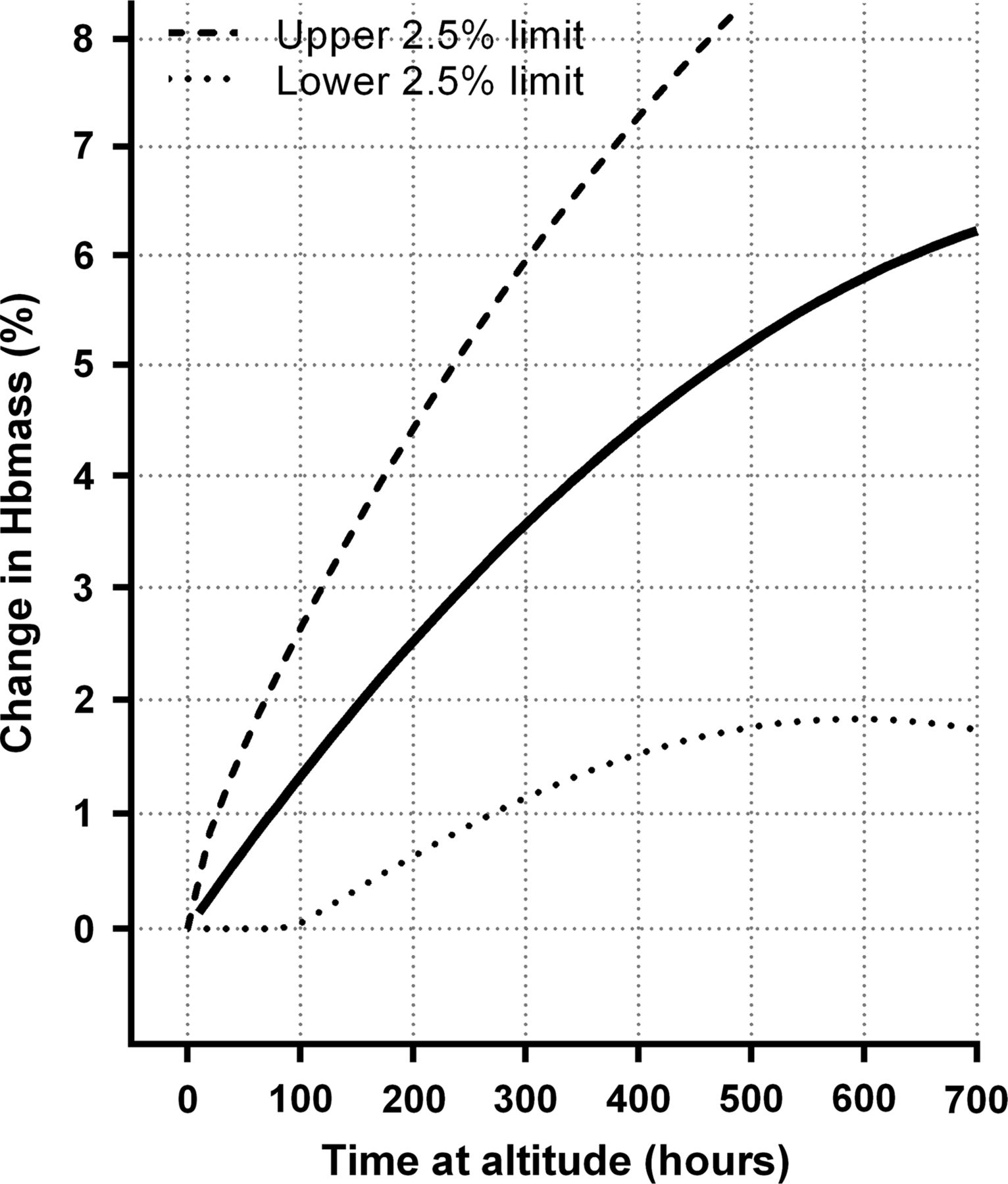
For the within-subject SDs obtained from differences in ln(Hbmass) between measurements taken prealtitude and while at altitude, a simple linear model in hours of exposure, with the SD equal to the estimated analytical SD for zero hours of exposure (the intercept), fitted the data reasonably well. Formal tests were carried out for departure from the forced intercept, for different responses to prealtitude to during altitude versus during altitude to during altitude, and for adding a quadratic term in altitude exposure, none of which were significant with p values of 0.331, 0.721 and 0.353, respectively. The results of this modelling are presented in figure 4, which gives estimated 95% prediction intervals for the ‘true’ increase in ln(Hbmass), for individuals, for different durations of altitude exposure. For example, while it is estimated that after 300 h of exposure the estimated median increase in Hbmass will be 3.52%, it is also estimated that 95% of individuals will have a ‘true’ increase in Hbmass of between 1.14% and 5.95%.
Estimated median and estimated between-subject ‘true’ change in haemoglobin mass (Hbmass) in response to altitude exposure. The solid line refers to the same quadratic model as in figure 1 with dashed lines being the upper and lower 95% individual response limits. Where the lower limit of the individual responses was estimated to be negative, it has been truncated at zero.
Discussion
The main findings of this meta-analysis are that Hbmass increases at approximately 1.1%/100 h of altitude exposure regardless of whether the exposure is classic altitude (>2100 m) or LHTL (∼3000 m), and that after a typical exposure of 300–400 h the increase above prealtitude values persists for ∼3 weeks. In addition, modelling suggests that 97.5% of individuals will have a ‘true’ increase in Hbmass after 100 h of altitude exposure.
During altitude
In 2004, Rusko et al38 combined the results of eight studies using simple linear regression and concluded that LHTL could increase Hbmass by approximately 0.3%/day of altitude. In 2009, Clark et al8 applied the same methodology as Rusko et al to more recent studies and estimated that Hbmass increases at a mean rate of 1%/100 h of exposure to an adequate LHTL altitude, but with large uncertainty of this estimate (SE of estimate ±3.5%). In a review of their own data, Levine and Stray-Gundersen39 concluded that 3 weeks of classic altitude exposure or LHTL for 12 h/day each generated an increase in RCV of ∼4%. The current meta-analysis confirms the estimate of ∼1%/100 h for the pooled data of LHTL and classic altitude; this finding contrasts with Rasmussen et al5 who concluded that below 3000 m of classic altitude there is no statistically significant increase in RCV within 4 weeks. The Monte Carlo simulation of Rasmussen et al5 (their table 3) indicates that a 1% increase in RCV at a 95% level of probability would take between 13–28 days and 18–31 days of classic and LHTL altitude exposure, respectively. Their simulation results contrast with the current estimate of ∼100 h, which equates to approximately 4 and 7 days for classic and LHTL, respectively, when the latter uses ∼14 h/day. What are the possible reasons for these contrasting time estimates?
Two explanations are tenable and both relate to noise/error in the data, since changes as small as 1% are below the analytical error of even the best methods. The first consideration is that Rasmussen et al5 selected RCV instead of Hbmass as their outcome variable. They needed to do so in order to standardise their data sources that were 44% from CO rebreathing, 37% from plasma dye dilution methods and 19% from radiolabelled albumin methods. Gore et al9 demonstrated that the typical error of RCV from CO rebreathing and Evans blue dye (a common plasma dye-dilution method) is ∼7%, with 90% confidence limits of ∼3–14% and 5–9%, respectively). In contrast, the corresponding typical error for Hbmass from CO rebreathing was estimated at 2.2% (90% confidence limits of 1.4% to 3.5%) for measures taken 1 day apart.9 Our best estimate of the analytical error for Hbmass from the current meta-analysis is 2.04% (95% confidence limits of 1.80% to 2.33%) for observations taken zero days apart. The approximate tripling of error using RCV instead of Hbmass relates partially to error propagation due to the extra steps of measuring the haemoglobin concentration and haematocrit required to estimate RCV and partially to the greater imprecision of dye-dilution methods.9 The second consideration is that relatively noisy data for RCV from a variety of sources will cloud small effects even with a statistically powerful meta-analytic approach as discussed by Rasmussen et al.5 They state that “the inclusion of results obtained with different methods may have increased the variance and reduced the power of the analysis.” Indeed, they also comment that the variability in their modelled increase in RCV across the pooled data set was ‘surprisingly large’, being an average of 49±240 mL/week. The median RCV of Rasmussen et al's participants was 2518 mL, so the uncertainty of ±240 mL equates to a variation of ±9.5% about the median RCV. This is consistent with the conclusion of the 2005 meta-analysis9 that RCV has ∼7% error for measures 1 day apart and closer to ∼8% for measures taken a month apart, as would be more typical with an altitude intervention. With 20% of Rasmussen et al's5 data from radiolabelled methods, one would have expected that their overall error may have been attenuated, but substantial noise is apparent in their data for the average estimates of the change in RCV for time spent at altitude.
Notwithstanding the large uncertainty, the average increase of 49 (±240) mL/week reported by Rasmussen et al5 corresponds to 1.95%/week of the median RCV, or an increase of 1.16%/100 h of altitude. This is similar to our estimate of 1.08%/100 h for Hbmass (table 2). Therefore, despite examining mostly different data sets, there is good agreement about the general magnitude of increase from altitude exposure between the current meta-analysis and that of Rasmussen et al5 albeit that the latter included substantially higher altitudes than the former.
Finally, data from lifelong altitude residents show that Hbmass will not increase indefinitely when athletes train at altitude; for instance, Schmidt et al40 found that the Hbmass relative to the body mass of cyclists from 2600 m was ∼10% higher than that of cyclists from sea level. So after some period of months, the increase that we report (figure 1) will plateau.41 ,42 Various models with such a plateau were tried but did not fit our data as well as the reported quadratic model, which should not be extrapolated beyond the range of our data; the maximum exposure to altitude among our data was 670 h. The fitted quadratic implies a maximum increase in Hbmass of 6.6% after 920 h, albeit that this result is quite likely specific to the data set that was examined and 920 h is well beyond the range of our data. Indeed, theoretically one would have expected that a model that would have best fitted our data would comprise a delay constant and two exponential functions, one for rapid changes and one for slow changes, which are typical of multicomponent acclimatisations. There should be a delay because of the time needed for increased red cell production43 and a steeper curve of increasing Hbmass during the first phase,29 before improved arterial oxygen content following a decrease in plasma volume44 and an increase in ventilation caused by water and bicarbonate excretion.45 Thereafter, a second slower phase of increasing Hbmass would be expected.3 However, multicomponent models of this sophistication did not fit our data better than the models we derived. More elaborate models would require more extensive data than were available, but our parsimonious linear model (a linear increase of ∼1%/100 h) is simple for practitioners to apply.
Postaltitude
The veracity of the estimated increase in Hbmass during altitude exposure is supported by the results posthypoxia from our current meta-analysis, with a significant increase of ∼3–4% evident following typical exposures to classic and LHTL altitude exposure. In addition, this is the first meta-analytic attempt to characterise the time course of Hbmass after altitude exposure. Our modelling indicated a ∼3% increase in Hbmass for up to 20 days post classic and LHTL altitude exposure. Prommer et al46 have most carefully characterised the time course of Hbmass in Kenyans living temporarily near sea level; they observed no discernible change in Hbmass for the first 14 days and then a significant (∼2.5%) decrease after 21 days, which was ∼3.3% in magnitude after 28 days and ∼6% after 40 days. However, one might expect that the time course for lifelong altitude residents might differ from that of athletes who had only sojourned to altitude for a few weeks.
Neocytolysis, the preferential destruction of young circulating RBCs (neocytes) by reticuloendothelial phagocytes,47 is considered the likely cause of the response after descent from altitude.48 Pottgiesser et al49 explored serum erythropoietin, serum ferritin, percentage of reticulocytes and Hbmass as indirect markers of neocytolysis in athletes subsequent to LHTL and concluded that there was evidence of rapid red blood cell destruction, at least in some athletes. The data of Pottgiesser et al are included in the current meta-analysis as part of Garvican et al14 but when pooled with the other available studies, the evidence for a rapid decrease in Hbmass is not present. A recent study of Bolivians transitioning from La Paz (3600 m) to near sea level for 6 days also reached the same conclusion; specifically, that Hbmass did not decrease rapidly for altitude natives during a few days near sea level.31 However, it needs to be acknowledged that for our meta-analysis there is a paucity of data in excess of 7 days posthypoxia; specifically, 19 of the 31 values (61%) used in this meta-analysis were for data collected within the first week postaltitude. In addition, the quality of the data was noticeably better (smaller SEs) for the data collected ≤14 days postaltitude, which adds supports to the confidence in our conclusion that the posthypoxia increase is significant. To better understand the time course of Hbmass postaltitude exposure, future research should focus particularly on generating data up to 4 weeks after exposure.
Variability of within-subject measurement
Measures less than or equal to a week apart were associated with a within-subject CV of ∼2%, which is very similar to both the 2.2% estimated in a previous meta-analysis for measures taken 1 day apart9 and the estimates of 1.9 and 2% for men and women, respectively, for measures taken on the same day.36 The most recent estimate of the CV of Hbmass of 1.6% for measures taken ∼12 days apart is even lower,18 which is much less than in the present study and may reflect successive refinements to the CO rebreathing method over time, such as higher doses of CO and more replicate measurements of carboxyhaemoglobin,16 as well as the use of custom quality control materials.18 In the current meta-analysis, the SD of paired observations increased over time for measures conducted more than 1 week apart, such that for measures 40 days apart the within-subject CV is ∼2.68%. It should be appreciated that the estimate of within-subject SD taken more than a few days apart includes biological and analytical components that are independent and additive.36 In the current meta-analysis, there was little evidence of biological variation for the first week, but thereafter the additional progressive increase in SD is evidence of biological variation. Sources of biological variation in Hbmass of athletes include illness, injury,50 training51 and energy intake.22
Of the 80 estimates of within-subject CV, there were 5 which exceeded 4%, Frese and Friedmann-Bette,28 Garvican et al,29 and Saunders et al,21 and the largest of these was nearly 6% (figure 3). The latter two of these studies provided 39 estimates of the within-subject CV and when using small samples (n<7), a range of estimates is expected by chance alone. For the >7-day estimate of within-subject CV of 2.5% of this meta-analysis, the 95% limits for a change (calculated as ±1.96×√2×2.5) between successive measures on an individual is from −6.9% to 6.9%, since both the first and second measures will be subject to error. So changes as large as ∼7% are likely between two measures of Hbmass just over a week apart, and will occur 5% of the time (ie, one in every 20 measures). Furthermore, one in every 100 measures for a control participants will quite likely show a random change as much as 9.1% (2.57×√2×2.5), even though the Hbmass is stable. Such data should not be discarded as outliers; they are the inevitable consequence of measurement imprecision.
Given that the 7-day within-subject CV is ∼2% (the vast majority of which is likely to be due to analytical errors), how can this meta-analysis conclude that the 1% increase in Hbmass after ∼100 h of altitude exposure is statistically significant? The estimated change after ∼100 h at altitude (1.33%, table 2) is about half the uncertainty of the measure. But with adequate sample sizes, and hence statistical power, even small changes can be detected from a conventional statistical approach. The current meta-analysis of multiple estimates of the change in Hbmass, derived from time series measurements using CO rebreathing, has provided the means to do so. Radiolabelled methods such as 51Cr to estimate RCV are the criterion, but it is not practical to make multiple measurements on healthy athletes before, during and after altitude exposure due to radiation concerns.9 Indeed, given the findings of this meta-analysis, it would be potentially unethical to use radiolabelled methods, which have similar measurement error to CO rebreathing.9
Between-subject ‘true’ response
Statistically removing the analytical component of error from the measured change in Hbmass from prealtitude to during altitude and while at altitude allows a method to approximate the ‘true’ between-individual responsiveness to altitude exposure—albeit that it is inexact (figure 4).37 Our analysis reveals that 97.5% of individuals will increase Hbmass by at least 1% after 300 h of exposure (equivalent to 12.5 days of classic altitude or 21.4 days of LHTL with 14 h/day of hypoxia); the corresponding upper limit is 6%. Although these estimates are relatively crude approximations, they imply that a 2-week camp at classic altitude will increase the Hbmass of most athletes. Therefore, with adequate preparation,52 coaches and athletes can undertake such short camps with confidence such that they will quite likely be worthwhile for most individuals. However, if measured changes in Hbmass after a 2-week altitude camp are greater than ∼5.5% (eg, 10%), this would be indicative of measurement imprecision, as described in the previous subsection, rather than a ‘true’ increase of this magnitude.
Limitations
The limitations of this study are as follows: (1) all but one of the LHTL studies used the same simulated altitude of 3000 m, (2) only one of the LHTL studies was conducted at terrestrial altitude,24 (3) there are relatively few data in excess of 7 days postaltitude exposure, (4) none of the studies used double-blind placebo interventions and (5) training data are not included. With respect to the latter point, Garvican et al51 have modelled that a 10% change in a 42-day training load is associated with a 1% change in Hbmass. Thus, for a typical 3-week altitude camp, a 20% increase in training load, which would be large for an elite athlete, might be associated with a 1% increase in Hbmass. However, for a classic altitude camp of 3 weeks, the mean estimated increase in Hbmass is 5.2%, so the majority of the increase is quite likely attributable to altitude per se. If, as is common practice, the training load was actually reduced during the altitude camp, then any increase in Hbmass could reasonably be attributed to the altitude stimulus. Finally, while laboratory or competition performance postaltitude is susceptible to placebo effects,53 it is not tenable that Hbmass can be influenced by belief.
Application
In a busy schedule of training and competition, athletes may not be able to afford the time for the recommended 3–4 week blocks of altitude training,6 instead opting for camps as short as 2 weeks.39 The results of this meta-analysis support the notion that a 2-week classic camp (336 h) may be sufficient to increase Hbmass by a mean of ∼3% and by at least 1% for 97.5% of athletes. Athletes have been using altitude training of various forms for many years54 and, given that a worthwhile increase in performance for an elite athlete is of the order of 0.3–0.4%,55 ,56 it is possible that they are attuned to small but important changes in their physiology that might improve race performance. As indicated by Jacobs,57 the possibility of type II errors (falsely accepting null findings due to modest statistical power) may cloud our interpretation of studies of altitude training, particularly when it comes to performance. Atkinson et al58 support this idea and state specifically that “statistical significance and non-significance can no longer be taken as sole evidence for the presence or absence of a practically meaningful effect.”
What are the new findings
-
The optimised carbon monoxide rebreathing method to determine haemoglobin mass (Hbmass) has an analytical error of ∼2%, which provides a sound basis to interpret changes in Hbmass of athletes exposed to moderate altitude.
-
During-altitude Hbmass increases by ∼1.1%/100 h of adequate altitude exposure, so when living and training on a mountain (classic altitude) for just 2 weeks, a mean increase of ∼3.4% is anticipated.
-
Living high and training low (LHTL) at 3000 m simulated altitude is just as effective as classic altitude training at ∼2320 m at increasing Hbmass, when the total hours of hypoxia are matched.
-
∼97.5% of adequately prepared athletes are likely to increase Hbmass by at least 1% after approximately 300 h of altitude exposure, either classic or LHTL. ‘Adequately prepared’ includes being free from injury or illness, not ‘overtrained’ and with iron supplementation.
How might it impact on clinical practice in the near future
-
For athletes with a busy training and competition schedule, altitude training camps as short as 2 weeks of classic altitude will quite likely increase Hbmass and most athletes can expect benefit.
-
Athletes, coaches and sport scientists can use altitude training with high confidence of an erythropoietic benefit, even if the subsequent performance benefits are more tenuous.
References
Footnotes
-
Contributors CJG participated in the conception and design, acquisition of data, analysis and interpretation of data, drafting the article and final approval. KS participated in the analysis and interpretation of data, drafting the article and final approval. LAG-L, PUS, CEH, EYR, NBW, SAC, BDM, BF-B, MN, TP and YOS participated in the conception and design, acquisition of data, critical revision of the article and final approval. WFS participated in the conception and design, acquisition of data, analysis and interpretation of data, critical revision of the article and final approval.
-
Competing interests None.
-
Provenance and peer review Not commissioned; externally peer reviewed.